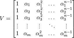
yourMATHsolver: Vandermonde matrix

In linear algebra, a Vandermonde matrix, named after Alexandre-Théophile Vandermonde, is a matrix with the terms of a geometric progression in each row, i.e., an m × n matrix

$V=\begin{bmatrix} 1 & \alpha_1 & \alpha_1^2 & \dots & \alpha_1^{n-1}\\ 1 & \alpha_2 & \alpha_2^2 & \dots & \alpha_2^{n-1}\\ 1 & \alpha_3 & \alpha_3^2 & \dots & \alpha_3^{n-1}\\ \vdots & \vdots & \vdots & \ddots &\vdots \\ 1 & \alpha_m & \alpha_m^2 & \dots & \alpha_m^{n-1} \end{bmatrix}$

$V_{i,j} = \alpha_i^{j-1} \,$

for all indices i and j. (Some authors use the transpose of the above matrix.)

The determinant of a square Vandermonde matrix (where m = n) can be expressed as:

$\det(V) = \prod_{1\le i<j\le n} (\alpha_j-\alpha_i).$

This is called the Vandermonde determinant or Vandermonde polynomial. If all the numbers

α i

are distinct, then it is non-zero.

The Vandermonde determinant is sometimes called the discriminant, although many sources, including this article, refer to the discriminant as the square of this determinant. Note that the Vandermonde determinant is alternating in the entries, meaning that permuting the

α i

by an odd permutation changes the sign, while permuting them by an even permutation does not change the value of the determinant. It thus depends on the order, while its square (the discriminant) does not depend on the order.

When two or more α_i are equal, the corresponding polynomial interpolation problem (see below) is underdetermined. In that case one may use a generalization called confluent Vandermonde matrices, which makes the matrix non-singular while retaining most properties. If α_i = α_i + 1 = ... = α_i+k and α_i ≠ α_i − 1, then the (i + k)th row is given by

$V_{i+k,j} = \begin{cases} 0, & \text{if } j \le k; \\ \frac{(j-1)!}{(j-k-1)!} \alpha_i^{j-k-1}, & \text{if } j > k. \end{cases}$

The above formula for confluent Vandermonde matrices can be readily derived by letting two parameters

α i

and

α j

go arbitrarily close to each other. The difference vector between the rows corresponding to

α i

and

α j

scaled to a constant yields the above equation (for k = 1). Similarly, the cases k > 1 are obtained by higher order differences. Consequently, the confluent rows are derivatives of the original Vandermonde row.

Properties

Using the Leibniz formula for the determinant,

$\det(V) = \sum_{\sigma \in S_n} \sgn(\sigma) \prod_{i = 1}^n \alpha_i^{\sigma(i)-1},$

where S_n denotes the set of permutations of $\mathbb{Z} \cap [1, n]$ , and sgn(σ) denotes the signature of the permutation σ, we can rewrite the Vandermonde determinant as

$\prod_{1\le i<j\le n} (\alpha_j-\alpha_i) = \sum_{\sigma \in S_n} \sgn(\sigma) \prod_{i = 1}^n \alpha_i^{\sigma(i)-1}.$

The Vandermonde polynomial (multiplied with the symmetric polynomials) generates all the alternating polynomials.

If m ≤ n, then the matrix V has maximum rank (m) if and only if all α_i are distinct. A square Vandermonde matrix is thus invertible if and only if the α_i are distinct; an explicit formula for the inverse is known.

Applications

The Vandermonde matrix evaluates a polynomial at a set of points; formally, it transforms coefficients of a polynomial $a_0+a_1x+a_2x^2+\cdots+a_{n-1}x^{n-1}$ to the values the polynomial takes at the points

α i .

The non-vanishing of the Vandermonde determinant for distinct points

α i

shows that, for distinct points, the map from coefficients to values at those points is a one-to-one correspondence, and thus that the polynomial interpolation problem is solvable with unique solution; this result is called the unisolvence theorem.

They are thus useful in polynomial interpolation, since solving the system of linear equations Vu = y for u with V an m × n Vandermonde matrix is equivalent to finding the coefficients u_jof the polynomial(s)

$P(x)=\sum_{j=0}^{n-1} u_j x^j$

of degree ≤ n − 1 which has (have) the property

$P(\alpha_i) = y_i \quad\text{for } i=1,\ldots, m. \,$

The Vandermonde matrix can easily be inverted in terms of Lagrange basis polynomials:each column is the coefficients of the Lagrange basis polynomial, with terms in increasing order going down. The resulting solution to the interpolation problem is called the Lagrange polynomial.

The Vandermonde determinant plays a central role in the Frobenius formula, which gives the character of conjugacy classes of representations of the symmetric group.

When the values

α k

range over powers of a finite field, then the determinant has a number of interesting properties: for example, in proving the properties of a BCH code.

Confluent Vandermonde matrices are used in Hermite interpolation.

A commonly known special Vandermonde matrix is the discrete Fourier transform matrix (DFT matrix), where the numbers α_i are chosen equal to the m different mth roots of unity.

The Vandermonde matrix diagonalizes a companion matrix.

Pages

Friday, January 27, 2012

Vandermonde matrix

No comments:

Post a Comment