Cramer's rule(Linear Algebra)

In linear algebra, Cramer's rule is a theorem, which gives an expression for the solution of a system of linear equations with as many equations as unknowns, valid in those cases where there is a unique solution. The solution is expressed in terms of the determinants of the (square) coefficient matrix and of matrices obtained from it by replacing one column by the vector of right hand sides of the equations. It is named after Gabriel Cramer (1704–1752), who published the rule in his 1750 Introduction à l'analyse des lignes courbes algébriques (Introduction to the analysis of algebraic curves), although Colin Maclaurin also published the method in his 1748 Treatise of Algebra (and probably knew of the method as early as 1729).


General Case

onsider a system of n linear equations for n unknowns, represented in matrix multiplication form as follows:

where the n by n matrix A has a nonzero determinant, and the vector  is the column vector of the variables.

Then the theorem states that in this case the system has a unique solution, whose individual values for the unknowns are given by:

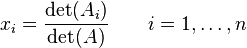
where A_i is the matrix formed by replacing the ith column of A by the column vector b.

The rule holds for systems of equations with coefficients and unknowns in any field, not just in the real numbers. It has recently been shown that Cramer's rule can be implemented in O(n³) time, which is comparable to more common methods of solving systems of linear equations, such as Gaussian elimination.

Proof

The proof for Cramer's rule is very simple; in fact, it uses just two properties of determinants: linearity with respect to any given column (taking for that column a linear combination of column vectors produces as determinant the corresponding linear combination of their determinants), and the fact that the determinant is zero whenever two columns are equal (the determinant is alternating in the columns).

Fix the index j of a column. Linearity means that if we consider only column j as variable (fixing the others arbitrarily), the resulting function Rⁿ → R (assuming matrix entries are in R) can be given by a matrix, with one row and n columns. In fact this is precisely what Laplace expansion does, writing det(A) = C₁a_1,j + … + C_na_n,j for certain coefficients C₁,…,C_n that depend on the columns of A other than column j (the precise expression for these cofactors is not important here). The value det(A) is then the result of applying the one-line matrixL_(j) = (C₁ C₂ … C_n) to column j of A. If L_(j) is applied to any other column k of A, then the result is the determinant of the matrix obtained from A by replacing column j by a copy of column k, which is 0 (the case of two equal columns).

Now consider a system of n linear equations in n unknowns , whose coefficient matrix is A, with det(A) assumed to be nonzero:

If one combines these equations by taking C₁ times the first equation, plus C₂ times the second, and so forth until C_n times the last, then the coefficient of x_j will becomeC₁a_1,j + … + C_na_n,j = det(A), while the coefficients of all other unknowns become 0; the left hand side becomes simply det(A)x_j. The right hand side is C₁b₁ + … + C_nb_n, which is L_(j)applied to the column vector b of the right hand sides b_i. In fact what has been done here is multiply the matrix equation A ⋅ x = b on the left by L_(j). Dividing by the nonzero number det(A) one finds the following equation, necessary to satisfy the system:

But by construction the numerator is determinant of the matrix obtained from A by replacing column j by b, so we get the expression of Cramers rule as necessary condition for a solution. The same procedure can be repeated for other values of j to find values for the other unknowns.

The only point that remains to prove is that these values for the unknowns, the only possible ones, to indeed together form a solution. But if the matrix A is invertible with inverse A⁻¹, then x = A⁻¹ ⋅ b will be a solution, thus showing its existence. To see that A is invertible when det(A) is nonzero, consider the n by n matrix M obtained by stacking the one-line matrices L_(j) on top of each other for j = 1, 2, …, n (this gives the adjugate matrix for A). It was shown that L_(j) ⋅ A = (0 … 0 det(A) 0 … 0) where det(A) appears at the position j; from this it follows that M ⋅ A = det(A)I_n. Therefore

completing the proof.

Finding inverse matrix

Let A be an n×n matrix. Then

where Adj(A) denotes the adjugate matrix of A, det(A) is the determinant, and I is the identity matrix. If det(A) is invertible in R, then the inverse matrix of A is

If R is a field (such as the field of real numbers), then this gives a formula for the inverse of A, provided det(A) ≠ 0. In fact, this formula will work whenever R is a commutative ring, provided that det(A) is a unit. If det(A) is not a unit, then A is not invertible.