Confidence intervals

In statistics, a confidence interval (CI) is a kind of interval estimate of a population parameter and is used to indicate the reliability of an estimate. It is an observed interval (i.e. it is calculated from the observations), in principle different from sample to sample, that frequently includes the parameter of interest, if the experiment is repeated. How frequently the observed interval contains the parameter is determined by the confidence level or confidence coefficient. More specifically, the meaning of the term "confidence level" is that, if confidence intervals are constructed across many separate data analyses of repeated (and possibly different) experiments, the proportion of such intervals that contain the true value of the parameter will approximately match the confidence level; this is guaranteed by the reasoning underlying the construction of confidence intervals.

Confidence intervals consist of a range of values (interval) that act as good estimates of the unknown population parameter. However, in rare cases, none of these values may cover the value of the parameter. The level of confidence of the confidence interval would indicate the probability that the confidence range captures this true population parameter given a distribution of samples. It does not describe any single sample. This value is represented by a percentage, so when we say, "we are 99% confident that the true value of the parameter is in our confidence interval", we express that 99% of the observed confidence intervals will hold the true value of the parameter. After a sample is taken, the population parameter is either in the interval made or not, there is no chance. The level of confidence is set by the researcher (not determined by data) . If a corresponding hypothesis test is performed, the confidence level corresponds with the level of significance, i.e. a 95% confidence interval reflects an significance level of 0.05, and the confidence interval contains the parameter values that, when tested, should not be rejected with the same sample. Greater levels of confidence give larger confidence intervals, and hence less precise estimates of the parameter. Confidence intervals of difference parameters not containing 0 imply that that there is a statistically significant difference between the populations.

Certain factors may affect the confidence interval size including size of sample, level of confidence, and population variability. A larger sample size normally will lead to a better estimate of the population parameter.

A confidence interval does not predict that the true value of the parameter has a particular probability of being in the confidence interval given the data actually obtained. (An interval intended to have such a property, called a credible interval, can be estimated using Bayesian methods; but such methods bring with them their own distinct strengths and weaknesses).

Introduction

Interval estimates can be contrasted with point estimates. A point estimate is a single value given as the estimate of a population parameter that is of interest, for example the mean of some quantity. An interval estimate specifies instead a range within which the parameter is estimated to lie. Confidence intervals are commonly reported in tables or graphs along with point estimates of the same parameters, to show the reliability of the estimates.

For example, a confidence interval can be used to describe how reliable survey results are. In a poll of election voting-intentions, the result might be that 40% of respondents intend to vote for a certain party. A 90% confidence interval for the proportion in the whole population having the same intention on the survey date might be 38% to 42%. From the same data one may calculate a 95% confidence interval, which might in this case be 36% to 44%. A major factor determining the length of a confidence interval is the size of the sample used in the estimation procedure, for example the number of people taking part in a survey.

Statistical hypothesis testing

Relationship with other statistical topics

Confidence intervals are closely related to statistical significance testing. For example, if for some estimated parameter θ one wants to test the null hypothesis that θ = 0 against the alternative that θ ≠ 0, then this test can be performed by determining whether the confidence interval for θ contains 0.

More generally, given the availability of a hypothesis testing procedure that can test the null hypothesis θ = θ₀ against the alternative that θ ≠ θ₀ for any value of θ₀, then a confidence interval with confidence level γ = 1 − α can be defined as containing any number θ₀ for which the corresponding null hypothesis is not rejected at significance level α.

In consequence, if the estimates of two parameters (for example, the mean values of a variable in two independent groups of objects) have confidence intervals at a given γ value that do not overlap, then the difference between the two values is significant at the corresponding value of α. However, this test is too conservative. If two confidence intervals overlap, the difference between the two means still may be significantly different.

Confidence region

Confidence regions generalize the confidence interval concept to deal with multiple quantities. Such regions can indicate not only the extent of likely sampling errors but can also reveal whether (for example) it is the case that if the estimate for one quantity is unreliable then the other is also likely to be unreliable. See also confidence bands.

In applied practice, confidence intervals are typically stated at the 95% confidence level. However, when presented graphically, confidence intervals can be shown at several confidence levels, for example 50%, 95% and 99%.

Practical example

A machine fills cups with margarine, and is supposed to be adjusted so that the content of the cups is 250 g of margarine. As the machine cannot fill every cup with exactly 250 g, the content added to individual cups shows some variation, and is considered a random variable X. This variation is assumed to be normally distributed around the desired average of 250 g, with a standard deviation of 2.5 g. To determine if the machine is adequately calibrated, a sample of n = 25 cups of margarine are chosen at random and the cups are weighed. The resulting measured masses of margarine are X₁, ..., X₂₅, a random sample from X.

To get an impression of the expectation μ, it is sufficient to give an estimate. The appropriate estimator is the sample mean:

The sample shows actual weights x₁, ..., x₂₅, with mean:

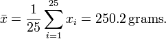
If we take another sample of 25 cups, we could easily expect to find mass values like 250.4 or 251.1 grams. A sample mean value of 280 grams however would be extremely rare if the mean content of the cups is in fact close to 250 grams. There is a whole interval around the observed value 250.2 grams of the sample mean within which, if the whole population mean actually takes a value in this range, the observed data would not be considered particularly unusual. Such an interval is called a confidence interval for the parameter μ. How do we calculate such an interval? The endpoints of the interval have to be calculated from the sample, so they are statistics, functions of the sample X₁, ..., X₂₅and hence random variables themselves.

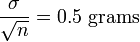
In our case we may determine the endpoints by considering that the sample mean X from a normally distributed sample is also normally distributed, with the same expectation μ, but with a standard error of:

By standardizing, we get a random variable:

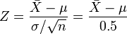
dependent on the parameter μ to be estimated, but with a standard normal distribution independent of the parameter μ. Hence it is possible to find numbers −z and z, independent of μ, between which Z lies with probability 1 − α, a measure of how confident we want to be.

We take 1 − α = 0.95, for example. So we have:

The number z follows from the cumulative distribution function, in this case the cumulative normal distribution function:

and we get:

In other words, the lower endpoint of the 95% confidence interval is:

and the upper endpoint of the 95% confidence interval is:

With the values in this example, the confidence interval is:

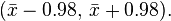
This might be interpreted as: with probability 0.95 we will find a confidence interval in which we will meet the parameter μ between the stochastic endpoints

and

This does not mean that there is 0.95 probability of meeting the parameter μ in the interval obtained by using the currently computed value of the sample mean,

Instead, every time the measurements are repeated, there will be another value for the mean X of the sample. In 95% of the cases μ will be between the endpoints calculated from this mean, but in 5% of the cases it will not be. The actual confidence interval is calculated by entering the measured masses in the formula. Our 0.95 confidence interval becomes:

In other words, the 95% confidence interval is between the lower endpoint 249.22 g and the upper endpoint 251.18 g.

As the desired value 250 of μ is within the resulted confidence interval, there is no reason to believe the machine is wrongly calibrated.

The calculated interval has fixed endpoints, where μ might be in between (or not). Thus this event has probability either 0 or 1. One cannot say: "with probability (1 − α) the parameter μ lies in the confidence interval." One only knows that by repetition in 100(1 − α) % of the cases, μ will be in the calculated interval. In 100α % of the cases however it does not. And unfortunately one does not know in which of the cases this happens. That is why one can say: "with confidence level100(1 − α) %, μ lies in the confidence interval."

The figure on the right shows 50 realizations of a confidence interval for a given population mean μ. If we randomly choose one realization, the probability is 95% we end up having chosen an interval that contains the parameter; however we may be unlucky and have picked the wrong one. We will never know; we are stuck with our interval.

Theoretical example

Suppose {X₁, ..., X_n} is an independent sample from a normally distributed population with (parameters) mean μ and variance σ². Let

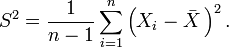
Where X is the sample mean, and S² is the sample variance. Then

has a Student's t-distribution with n − 1 degrees of freedom. Note that the distribution of T does not depend on the values of the unobservable parameters μ and σ²; i.e., it is a pivotal quantity. Suppose we wanted to calculate a 90% confidence interval for μ. Then, denoting c as the 95th percentile of this distribution,

(Note: "95th" and "0.9" are correct in the preceding expressions. There is a 5% chance that T will be less than −c and a 5% chance that it will be larger than +c. Thus, the probability that T will be between −c and +c is 90%.)

Consequently

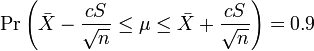
and we have a theoretical (stochastic) 90% confidence interval for μ.

After observing the sample we find values x for X and s for S, from which we compute the confidence interval

an interval with fixed numbers as endpoints, of which we can no longer say there is a certain probability it contains the parameter μ; either μ is in this interval or isn't.

Relation to Hypothesis Testing

While the formulations of the notions of confidence intervals and of statistical hypothesis testing are distinct they are in some senses related and to some extent complementary. While not all confidence intervals are constructed in this way, one general purpose approach to constructing confidence intervals is to define a 100(1 − α)% confidence interval to consist of all those values θ₀ for which a test of the hypothesis θ = θ₀ is not rejected at a significance level of 100α%. Such an approach may not always be available since it presupposes the practical availability of an appropriate significance test. Naturally, any assumptions required for the significance test would carry over to the confidence intervals.

It may be convenient to make the general correspondence that parameter values within a confidence interval are equivalent to those values that would not be rejected by a hypothesis test, but this would be dangerous. In many instances the confidence intervals that are quoted are only approximately valid, perhaps derived from "plus or minus twice the standard error", and the implications of this for the supposedly corresponding hypothesis tests are usually unknown.

It is worth noting, that the confidence interval for a parameter is not the same as the acceptance region of a test for this parameter, as is sometimes thought. How could it be? The confidence interval is part of the parameter space, whereas the acceptance region is part of the sample space. For the same reason the confidence level is not the same as the complementary probability of the level of significance.