yourMATHsolver: Green's theorem

In mathematics, Green's theorem gives the relationship between a line integral around a simple closed curve C and a double integral over the plane region D bounded by C. It is the two-dimensional special case of the more general Stokes' theorem, and is named after British mathematician George Green.

Let C be a positively oriented, piecewise smooth, simple closed curve in the plane $\mathbb{R}$ ², and let D be the region bounded by C. If L and M are functions of (x, y) defined on an open region containing D and have continuous partial derivatives there, then

$\oint_{C} (L\, \mathrm{d}x + M\, \mathrm{d}y) = \iint_{D} \left(\frac{\partial M}{\partial x} - \frac{\partial L}{\partial y}\right)\, \mathrm{d}x\, \mathrm{d}y.$

For positive orientation, an arrow pointing in the counterclockwise direction may be drawn in the small circle in the integral symbol.

In physics, Green's theorem is mostly used to solve two-dimensional flow integrals, stating that the sum of fluid outflows at any point inside a volume is equal to the total outflow summed about an enclosing area. In plane geometry, and in particular, area surveying, Green's theorem can be used to determine the area and centroid of plane figures solely by integrating over the perimeter.

Proof when D is a simple region

The following is a proof of the theorem for the simplified area D, a type I region where C₂ and C₄ are vertical lines. A similar proof exists for when D is a type II region where C₁ and C₃ are straight lines. The general case can be deduced from this special case by approximating the domain D by a union of simple domains.

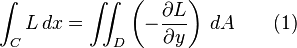
If it can be shown that

$\int_{C} L\, dx = \iint_{D} \left(- \frac{\partial L}{\partial y}\right)\, dA\qquad\mathrm{(1)}$

and

$\int_{C} M\, dy = \iint_{D} \left(\frac{\partial M}{\partial x}\right)\, dA\qquad\mathrm{(2)}$

are true, then Green's theorem is proven in the first case.

Define the type I region D as pictured on the right by:

$D = \{(x,y)|a\le x\le b, g_1(x) \le y \le g_2(x)\}$

where g₁ and g₂ are continuous functions on [a, b]. Compute the double integral in (1):

$\begin{align} \iint_D \frac{\partial L}{\partial y}\, dA & =\int_a^b\,\int_{g_1(x)}^{g_2(x)} \frac{\partial L}{\partial y} (x,y)\,dy\,dx \\ & = \int_a^b \Big\{L(x,g_2(x)) - L(x,g_1(x)) \Big\} \, dx\qquad\mathrm{(3)} \end{align}$

Now compute the line integral in (1). C can be rewritten as the union of four curves: C₁, C₂, C₃, C₄.

With C₁, use the parametric equations: x = x, y = g₁(x), a ≤ x ≤ b. Then

$\int_{C_1} L(x,y)\, dx = \int_a^b L(x,g_1(x))\, dx$

With C₃, use the parametric equations: x = x, y = g₂(x), a ≤ x ≤ b. Then

$\int_{C_3} L(x,y)\, dx = -\int_{-C_3} L(x,y)\, dx = - \int_a^b L(x,g_2(x))\, dx$

The integral over C₃ is negated because it goes in the negative direction from b to a, as C is oriented positively (counterclockwise). On C₂ and C₄, x remains constant, meaning

$\int_{C_4} L(x,y)\, dx = \int_{C_2} L(x,y)\, dx = 0$

Therefore,

$\begin{align} \int_{C} L\, dx & = \int_{C_1} L(x,y)\, dx + \int_{C_2} L(x,y)\, dx + \int_{C_3} L(x,y)\, dx + \int_{C_4} L(x,y)\, dx \\ & = -\int_a^b L(x,g_2(x))\, dx + \int_a^b L(x,g_1(x))\, dx\qquad\mathrm{(4)} \end{align}$

Combining (3) with (4), we get (1). Similar computations give (2).

Pages

Friday, January 13, 2012

Green's theorem

No comments:

Post a Comment