The Pirate Game

The pirate game is a simple mathematical game. It illustrates how, if assumptions conforming to a homo economicus model of human behaviour hold, outcomes may be surprising. It is a multi-player version of the ultimatum game.

The Game

There are 5 rational pirates, A, B, C, D and E. They find 100 gold coins. They must decide how to distribute them.

The pirates have a strict order of seniority: A is superior to B, who is superior to C, who is superior to D, who is superior to E.

The pirate world's rules of distribution are thus: that the most senior pirate should propose a distribution of coins. The pirates, including the proposer, then vote on whether to accept this distribution. If the proposed allocation is approved by a majority or a tie vote, it happens. If not, the proposer is thrown overboard from the pirate ship and dies, and the next most senior pirate makes a new proposal to begin the system again.

Pirates base their decisions on three factors. First of all, each pirate wants to survive. Second, given survival, each pirate wants to maximize the number of gold coins he receives. Third, each pirate would prefer to throw another overboard, if all other results would otherwise be equal. The pirates do not trust each other, and will neither make nor honor any promises between pirates apart from the main proposal.

Cauchy Sequences

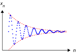
In mathematics, a Cauchy sequence , named after Augustin-Louis Cauchy, is a sequence whose elements become arbitrarily close to each otheras the sequence progresses. More precisely, given any small positive distance, all but a finite number of elements of the sequence are less than that given distance from each other.

The utility of Cauchy sequences lies in the fact that in a complete metric space (one where all such sequences are known to converge to a limit), the criterion for convergence depends only on the terms of the sequence itself. This is often exploited in algorithms, both theoretical and applied, where an iterative process can be shown relatively easily to produce a Cauchy sequence, consisting of the iterates.

The notions above are not as unfamiliar as they might at first appear. The customary acceptance of the fact that any real number x has a decimal expansion is an implicit acknowledgment that a particular Cauchy sequence of rational numbers (whose terms are the successive truncations of the decimal expansion of x) has the real limit x. In some cases it may be difficult to describe x independently of such a limiting process involving rational numbers.

Generalizations of Cauchy sequences in more abstract uniform spaces exist in the form of Cauchy filter and Cauchy net.

An Introduction to Group Theory

How to diagonalize a matrix

Consider a matrix

This matrix has eigenvalues

So A is a 3-by-3 matrix with 3 different eigenvalues, therefore it is diagonalizable. Note that if there are exactly n distinct eigenvalues in an n×n matrix then this matrix is diagonalizable.

These eigenvalues are the values that will appear in the diagonalized form of matrix , so by finding the eigenvalues of  we have diagonalized it. We could stop here, but it is a good check to use the eigenvectors to diagonalize .

Identity Theorem

In complex analysis, a branch of mathematics, the identity theorem for holomorphic functions states: given functions f and g holomorphic on a connected open set D, if f = g on some neighborhood of z that is in D, then f = g on D. Thus a holomorphic function is completely determined by its values on a (possibly quite small) neighborhood in D. This is not true for real-differentiable functions. In comparison, holomorphy, or complex-differentiability, is a much more rigid notion. Informally, one sometimes summarizes the theorem by saying holomorphic functions are "hard" (as opposed to, say, continuous functions which are "soft").

The underpinning fact from which the theorem is established is the developability of a holomorphic function into its Taylor series.

Proof

The connectedness assumption on the domain D is necessary and is in fact key to a short proof given here (obviously, if D consists of two disjoint open sets, the result does not hold). Under this assumption, since we are given that the set is not empty, topologically the claim amounts to that f and g coincide on a set that is both open and closed.

The closedness is immediate from the continuity of f and g.

Therefore, the main issue is to show that the set on which f = g is an open set.

Because a holomorphic function can be represented by its Taylor series everywhere on its domain, it is sufficient to consider the set

Suppose w lies in S. Then, because the Taylor series of f and g at w have non-zero radius of convergence, the open disk B_r(w) also lies in S for some r. (In fact, r can be anything less than the distance from w to the boundary of D). This shows S is open and proves the theorem.

The 4 Puzzle

The 4 Puzzle

Butterfly Curve and Variations

Butterfly Curve and Variations

Liouville's theorem (complex analysis)

In complex analysis, Liouville's theorem, named after Joseph Liouville, states that every bounded entire function must be constant. That is, every holomorphic function f for which there exists a positive number M such that |f(z)| ≤ M for all z in C is constant.

The theorem is considerably improved by Picard's little theorem, which says that every entire function whose image omits at least two complex numbers must be constant.

Proof

The theorem follows from the fact that holomorphic functions are analytic. Since f is entire, it can be represented by its Taylor series about 0

where (by Cauchy's integral formula)

and C_r is the circle about 0 of radius r > 0. We can estimate directly

where in the second inequality we have invoked the assumption that |f(z)| ≤ M for all z and the fact that |z|=r on the circle C_r. But the choice of r in the above is an arbitrary positive number. Therefore, letting r tend to infinity (we let r tend to infinity since f is analytic on the entire plane) gives a_k = 0 for all k ≥ 1. Thus f(z) = a₀ and this proves the theorem.

Confidence intervals

In statistics, a confidence interval (CI) is a kind of interval estimate of a population parameter and is used to indicate the reliability of an estimate. It is an observed interval (i.e. it is calculated from the observations), in principle different from sample to sample, that frequently includes the parameter of interest, if the experiment is repeated. How frequently the observed interval contains the parameter is determined by the confidence level or confidence coefficient. More specifically, the meaning of the term "confidence level" is that, if confidence intervals are constructed across many separate data analyses of repeated (and possibly different) experiments, the proportion of such intervals that contain the true value of the parameter will approximately match the confidence level; this is guaranteed by the reasoning underlying the construction of confidence intervals.

Confidence intervals consist of a range of values (interval) that act as good estimates of the unknown population parameter. However, in rare cases, none of these values may cover the value of the parameter. The level of confidence of the confidence interval would indicate the probability that the confidence range captures this true population parameter given a distribution of samples. It does not describe any single sample. This value is represented by a percentage, so when we say, "we are 99% confident that the true value of the parameter is in our confidence interval", we express that 99% of the observed confidence intervals will hold the true value of the parameter. After a sample is taken, the population parameter is either in the interval made or not, there is no chance. The level of confidence is set by the researcher (not determined by data) . If a corresponding hypothesis test is performed, the confidence level corresponds with the level of significance, i.e. a 95% confidence interval reflects an significance level of 0.05, and the confidence interval contains the parameter values that, when tested, should not be rejected with the same sample. Greater levels of confidence give larger confidence intervals, and hence less precise estimates of the parameter. Confidence intervals of difference parameters not containing 0 imply that that there is a statistically significant difference between the populations.

Certain factors may affect the confidence interval size including size of sample, level of confidence, and population variability. A larger sample size normally will lead to a better estimate of the population parameter.

A confidence interval does not predict that the true value of the parameter has a particular probability of being in the confidence interval given the data actually obtained. (An interval intended to have such a property, called a credible interval, can be estimated using Bayesian methods; but such methods bring with them their own distinct strengths and weaknesses).

The Gaussian Integral

The Gaussian integral, also known as the Euler–Poisson integral is the integral of the Gaussian function e^−x2 over the entire real line. It is named after the German mathematician and physicist Carl Friedrich Gauss. The integral is:

This integral has wide applications. For example, with a slight change of variables it is used to compute the normalizing constant of the normal distribution. The same integral with finite limits is closely related both to the error function and the cumulative distribution function of the normal distribution.

Although no elementary function exists for the error function, as can be proven by the Risch algorithm, the Gaussian integral can be solved analytically through the tools of calculus. That is, there is no elementary indefinite integral for , but the definite integral  can be evaluated.

The Gaussian integral is encountered very often in physics and numerous generalizations of the integral are encountered in quantum field theory.

Poincaré Hyperbolic Disk

The Poincaré hyperbolic disk is a two-dimensional space having hyperbolic geometry defined as the disk , with hyperbolic metric

The Poincaré disk is a model for hyperbolic geometry in which a line is represented as an arc of a circle whose ends are perpendicular to the disk's boundary (and diameters are also permitted). Two arcs which do not meet correspond to parallel rays, arcs which meet orthogonally correspond to perpendicular lines, and arcs which meet on the boundary are a pair of limits rays. The illustration above shows a hyperbolic tessellation similar to M. C. Escher's Circle Limit IV (Heaven and Hell) (Trott 1999, pp. 10 and 83).

Integrals of trigonometric functions(Table)

The following is a list of integrals (antiderivative functions) of trigonometric functions.

Curvilinear Coordinates

In geometry, curvilinear coordinates are a coordinate system for Euclidean space in which the coordinate lines may be curved. These coordinates may be derived from a set of Cartesian coordinates by using a transformation that is locally invertible (a one-to-one map) at each point. This means that one can convert a point given in a Cartesian coordinate system to its curvilinear coordinates and back. The name curvilinear coordinates, coined by the French mathematician Lamé, derives from the fact that the coordinate surfaces of the curvilinear systems are curved.

Markov Chain

A Markov chain, named after Andrey Markov, is a mathematical system that undergoes transitions from one state to another, between a finite or countable number of possible states. It is a random process characterized as memoryless: the next state depends only on the current state and not on the sequence of events that preceded it. This specific kind of "memorylessness" is called the Markov property. Markov chains have many applications as statistical models of real-world processes.

Two envelopes problem

The two envelopes problem, also known as the exchange paradox, is a brain teaser, puzzle or paradox in logic, philosophy, probability and recreational mathematics, of special interest in decision theory and for the Bayesian interpretation of probability theory. Historically, it arose as a variant of the necktie paradox.

A statement of the problem starts with:

Let us say you are given two indistinguishable envelopes, each of which contains a positive sum of money. One envelope contains twice as much as the other. You may pick one envelope and keep whatever amount it contains. You pick one envelope at random but before you open it you are offered the possibility to take the other envelope instead.

It is possible to give arguments that show that it will be to your advantage to swap envelopes by showing that your expected return on swapping exceeds the sum in your envelope. This leads to the logical absurdity that it is beneficial to continue to swap envelopes indefinitely.

A large number of different solutions have been proposed. The usual scenario is that one writer proposes a solution that solves the problem as stated, but then some other writer discovers that by altering the problem a little the paradox is brought back to life again. In this way a family of closely related formulations of the problem is created which are then discussed in the literature.

It is quite common for authors to claim that the solution to the problem is easy, even elementary. However, when investigating these elementary solutions they are not always the same conclusions from one author to the next. Recently, several new papers are published every year regarding the problem and introducing new conclusions. Occasionally, new variants of the problem are introduced.